profile

Synopsis

Analyse a JSONL sample manifest produced by list and produce a Bloom-filter span profile.

USAGE

kmhelpers profile [OPTIONS] LIST_OUTPUT

Argument	Description
`LIST_OUTPUT`	JSONL sample manifest produced by `list` (required)
`-o, --output DIR`	Output directory for results (required)
`-g, --group N`	Partition Bloom Filters into `N` storage-balanced groups and overlay on plot (default: 20)
`-b, --base FLOAT`	Base for span bucket boundaries (default: 1.1); use values like 1.1 or 2.0 to widen or narrow bucket granularity

I/O

Input: JSONL sample manifest produced by list
Output: profile.yaml, groups.png in output directory (-o)

Advanced Options

Option	Description
`-fp, --false-positive-rate FLOAT`	Target Bloom-filter false-positive rate (default: 0.25)

Output Files

File	Description
`profile.yaml`	Natural distribution and storage-balanced grouped profile(s)
`groups.png`	Span combination analysis plots

Description

A span is an integer s = floor(log_base(n)), where n is the number of distinct \(k\)-mers in a sample and base controls bucket granularity (default: 2). It identifies the Bloom-filter size class required to index that sample at the target false-positive rate.

Span assignment diagram

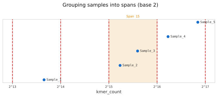
The figure above illustrates span assignment for five samples: each sample is placed on the k-mer count axis and falls into the bucket delimited by consecutive powers of the base. Here, samples whose k-mer count falls between \(2^{15}\) and \(2^{16}\) are assigned to Span 15.

A span profile is the distribution of samples across spans, together with candidate groupings of those spans into sub-indices. Fewer spans means fewer index files opened at query time, which improves query performance on I/O-bound storage.

profile reads \(k\)-mer counts from a JSONL file produced by list, assigns each sample to its span, and writes a CSV summary, a profile YAML, and a distribution plot to the output directory. Samples without a kmer_count field are skipped.

False-positive rate - a higher rate reduces Bloom-filter size and therefore disk footprint. At query time the findere algorithm compensates by querying \((k+z)\)-mers, reducing the effective FP rate to \(p^z\). Recommended: build with --fp 0.25 (default), query with -z 6, giving \(0.25^6 \approx 0.024\,\%\) effective FP rate.

Grouping - use -g N to merge spans into N storage-balanced sub-indices. Fewer sub-indices reduce the number of partition files opened per query. The grouping is overlaid on the distribution plot for visual inspection.

Examples

# Profile with default settings
kmhelpers profile samples.jsonl -o ./profile_output

# Use a stricter false-positive rate
kmhelpers profile samples.jsonl -o ./profile_output -fp 0.05

# Force a specific number of span groups
kmhelpers profile samples.jsonl -o ./profile_output -g 3

# Use a finer bucket granularity
kmhelpers profile samples.jsonl -o ./profile_output -b 1.5